A Python-based Eigensolver for Tanabe-Sugano & Energy-Correlation Diagrams
Interactive visualization of d-orbital splitting in transition metal complexes






🚀 Quick Start • ✨ Features • 📖 Documentation • 🎨 Examples • 🤝 Contributing
- Overview
- Quick Start
- Features
- Usage
- Examples
- Interactive Diagrams
- Scientific Background
- Contributing
- Citation
- License
TanabeSugano is a comprehensive Python package for calculating and visualizing Tanabe-Sugano and Energy-Correlation diagrams for d2-d8 transition metal ions. Based on the pioneering work of Yukito Tanabe and Satoru Sugano, this tool provides both computational accuracy and interactive visualization capabilities.
- 🎯 Accurate Calculations - Based on rigorous quantum mechanical principles
- 📊 Beautiful Visualizations - Generate publication-quality diagrams
- 🔄 Interactive Exploration - Explore diagrams with Plotly integration
- 🚀 Easy to Use - Simple CLI and Python API
- 📱 Cloud-Ready - Run in Google Colab or locally
Choose your preferred installation method:
# 📦 Install from PyPI (recommended)
pip install TanabeSugano

# 🔧 Install with interactive plotting support
pip install TanabeSugano[plotly]

# 🤖 Install with MCP server support (Claude Desktop, Cursor, VS Code, …)
pip install TanabeSugano[mcp]

# 🌐 Install from GitHub (latest development version)
pip install git+https://github.com/Anselmoo/TanabeSugano.git
Note: TanabeSugano now uses the
uv_buildbackend and requires Python ≥ 3.12.
Generate a Tanabe-Sugano diagram in seconds:
# Generate diagram for d6 configuration
tanabesugano -d 6

# Customize parameters
tanabesugano -d 6 -Dq 8000 -B 860 1.0 -C 3850 1.0
🎮 Try it now:
|
|
|
|
🔧 View all CLI options
tanabesugano --help

usage: __main__.py [-h] [-d D] [-Dq DQ] [-cut CUT] [-B B B] [-C C C] [-n N]
               [-ndisp] [-ntxt] [-slater]

optional arguments:
  -h, --help     show this help message and exit
  -d D           Number of unpaired electrons (default d5)
  -Dq DQ         10Dq crystal field splitting (default 10Dq = 8065 cm-)
  -cut CUT       10Dq crystal field splitting (default 10Dq = 8065 cm-)
  -B B B         Racah Parameter B and the corresponding reduction (default B = 860 cm- * 1.)
  -C C C         Racah Parameter C and the corresponding reduction (default C = 4.477*860 cm- * 1.)
  -n N           Number of roots (default nroots = 500)
  -ndisp         Plot TS-diagram (default = on)
  -ntxt          Save TS-diagram and dd energies (default = on)
  -slater        Using Slater-Condon F2,F4 parameter instead Racah-Parameter B,C (default = off)
  -v, --version  Print version number and exit
-html Save TS-diagram and dd energies (default = on)from tanabesugano import TanabeSugano
# Create a d6 configuration
ts = TanabeSugano(d=6, Dq=8065, B=860, C=3850)
# Generate and display diagram
ts.plot()
# Export to HTML for interactive use
ts.export_html('d6_diagram.html')High-quality diagram for d6 configuration with B = 860 cm⁻¹ and C = 3850 cm⁻¹:

Figure: Tanabe-Sugano diagram showing energy levels as a function of crystal field strength
Interactive diagram for d6 with Slater-Condon parameters F² = 1065 cm⁻¹ and F⁴ = 5120 cm⁻¹:
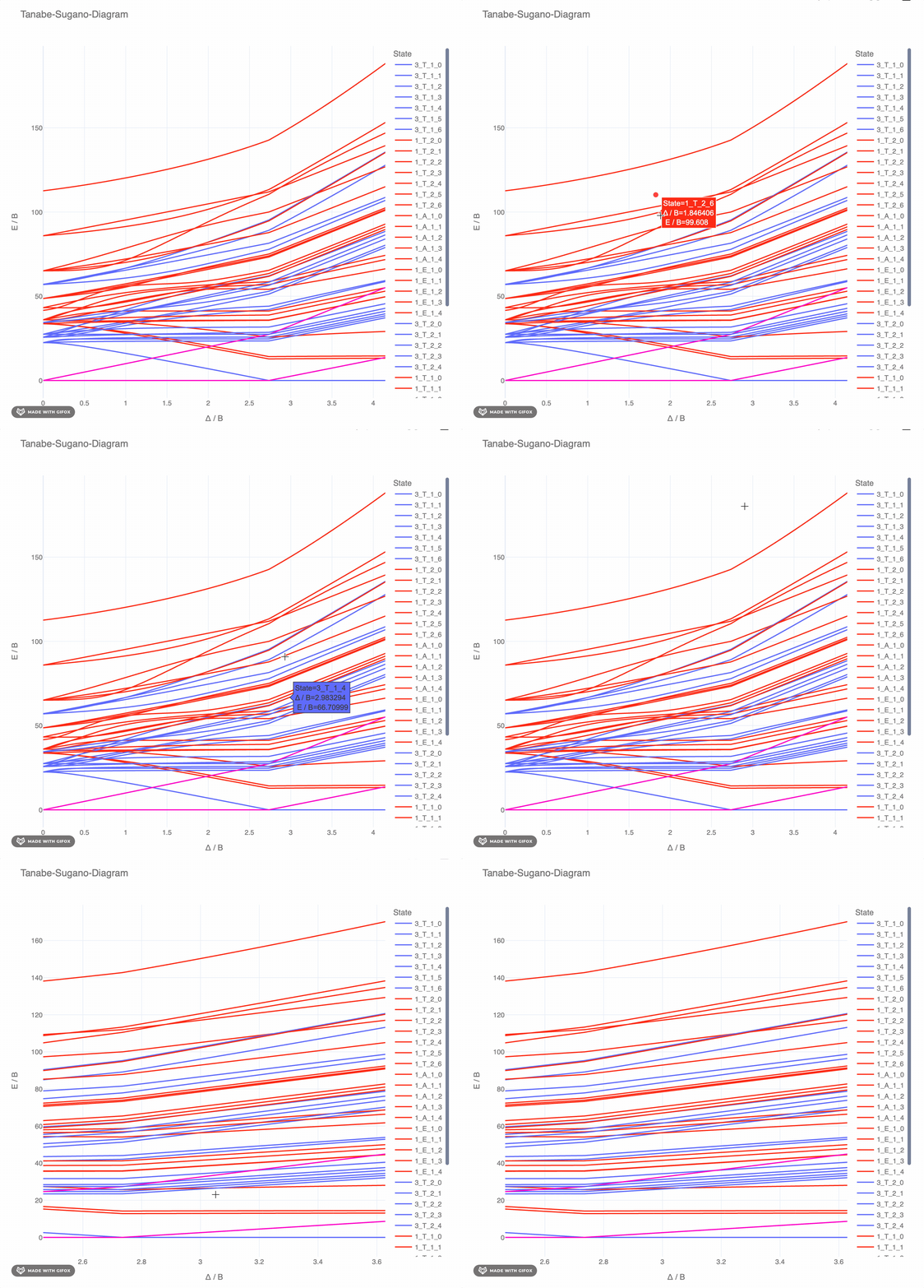
Figure: Interactive diagram with hover tooltips and zoom capabilities
✨ NEW: Explore all Tanabe-Sugano diagrams online!
All diagrams (d² through d⁸) are now available on our interactive GitHub Pages site with full Plotly integration:
No installation required - just click and explore!
TanabeSugano ships an optional Model Context Protocol server so AI assistants can compute diagrams, evaluate term symbols, and render plots as first-class tools.
pip install "TanabeSugano[mcp]"
# or with uv:
uv add "TanabeSugano[mcp]"Add to claude_desktop_config.json:
{
  "mcpServers": {
    "tanabesugano": {
      "command": "uvx",
      "args": ["--from", "tanabesugano[mcp]", "tanabesugano-mcp"]
    }
  }
}Every release attaches a tanabesugano-<version>.mcpb artifact (built by the Build .mcpb package workflow) that Claude Desktop can install in one step — drag the file onto the Claude Desktop window.
| Tool | Description |
|---|---|
ts_supported_configs |
List supported d-configurations (d²–d⁸). |
ts_terms_table_data |
All eigenvalues at one (Dq, B, C), sorted ascending with multiplicity (machine-readable rows). |
ts_fit_spectrum |
Fit observed UV-Vis absorption peaks → Dq and Racah B. |
ts_nephelauxetic |
Interpret a fitted B as metal-ligand covalency (nephelauxetic β). |
ts_plot_png |
Matplotlib PNG plot (cheap default for any client). |
ts_plot_view |
Interactive Chart.js line plot (capable clients only). |
ts_explain |
One-paragraph ground-state description. |
Note.
ts_computeandts_diagram(raw nested-dict eigenvalue payloads) were removed because the output was unusable without further rendering — Claude's "next steps" devolved into "save to CSV / render PNG" suggestions the client cannot execute. Usets_compute_app/ts_diagram_appfor in-chat tables and charts, orts_terms_table_datafor machine-readable rows.
| App | Description |
|---|---|
ts_dashboard_app |
Overview of all d²–d⁸ with ground terms, example ions, matrix sizes, and a concrete absorption-band number per configuration. |
ts_compute_app |
Sorted DataTable of every eigenvalue at one (Dq, B, C). Replaces the raw ts_compute. |
ts_diagram_app |
Full Tanabe-Sugano diagram as an interactive Chart.js line plot. |
ts_compare_app |
Multiple d-configurations overlaid on one shared Chart.js plot. |
ts_overlay_app |
Overlay multiple d-configurations on one shared chart. |
ts_oxidation_landscape_app |
Every eigenvalue of d²–d⁸ at fixed (Dq, B, C): style="scatter" (default) renders discrete dots per d-count, style="density" renders a Gaussian-broadened 2D heatmap (control σ via broadening_cm). |
ts_orgel_diagram_app |
Orgel diagram — E (cm⁻¹) vs Δ (cm⁻¹), the classic unnormalised companion to ts_diagram_app. d²/d³/d⁸ render smoothly; d⁴–d⁷ show the HS↔LS kink. |
ts_spin_crossover_app |
For d⁴/d⁵/d⁶/d⁷ only: ground-term energy of the candidate HS and LS curves vs Δ with the critical Dq annotated. Returns the numeric critical_Dq_cm1. |
ts_correlation_diagram_app |
Three-axis correlation diagram (free ion ↔ weak field ↔ strong field) — the classical Tsuchida/Cotton pedagogical bridge between free-ion term symbols and strong-field t₂g^x e_g^y configurations. |
ts_spectrum_app |
Simulated Lorentzian UV-Vis spectrum (spin-allowed + spin-forbidden). |
ts_reverse_fit_app |
Grid-search Dq and B to best-fit observed peak positions. |
ts_ratio_fit_app |
Derive Dq and B from 2–3 measured bands via the ratio method. |
Prompts: tanabesugano_why (discovery context) and tanabesugano_explain_complex (guided spectrum interpretation from measured absorption peaks).
Resources at tanabesugano://version, tanabesugano://configs, tanabesugano://config/{d} provide static metadata.
This implementation is based on the seminal work of Yukito Tanabe and Satoru Sugano:
📖 Paper I: Absorption Spectra of Complex Ions
Authors: Yukito Tanabe, Satoru Sugano Journal: Journal of the Physical Society of Japan, Vol. 9, pp. 753-766 (1954) DOI: 10.1143/JPSJ.9.753 Link: https://journals.jps.jp/doi/10.1143/JPSJ.9.753
📖 Paper II: Absorption Spectra of Complex Ions
Authors: Yukito Tanabe, Satoru Sugano Journal: Journal of the Physical Society of Japan, Vol. 9, pp. 766-779 (1954) DOI: 10.1143/JPSJ.9.766 Link: https://journals.jps.jp/doi/10.1143/JPSJ.9.766
📖 Paper III: Calculation of Crystalline Field Strength
Authors: Yukito Tanabe, Satoru Sugano Journal: Journal of the Physical Society of Japan, Vol. 11, pp. 864-877 (1956) DOI: 10.1143/JPSJ.11.864 Link: https://journals.jps.jp/doi/10.1143/JPSJ.11.864
We welcome contributions! Whether you're fixing bugs, adding features, or improving documentation, your help is appreciated.
- 📖 Read our Contributing Guide
- 🐛 Report issues on GitHub Issues
- 💡 Suggest features or improvements
- 🔧 Submit pull requests
If you use TanabeSugano in your research, please cite:
@software{tanabesugano,
  author       = {Anselm Hahn},
  title        = {TanabeSugano: Python-based Eigensolver for Tanabe-Sugano Diagrams},
  year         = {2024},
  publisher    = {Zenodo},
  doi          = {10.5281/zenodo.206847682},
  url          = {https://github.com/Anselmoo/TanabeSugano}
}This project is licensed under the MIT License - see the LICENSE file for details.
Made with ❤️ for the scientific community
⭐ Star us on GitHub — it helps!